Volatility and The Option Greeks
Introduction to Standard Deviation
Introduction to Standard Deviation
Imagine a group of friends embarking on a road trip from their hometown to a vacation destination. Each friend decides to drive their own car, and they all start from the same point.
Now let's say that each friend has a different driving style. Some friends prefer to drive at a steady pace, maintaining a constant speed throughout the journey. Others might drive more erratically, speeding up and slowing down frequently.
As they travel, the distance between each car and the destination fluctuates based on their individual driving styles. The standard deviation in this scenario would represent how much each friend's distance deviates from the average distance traveled by the group.
For example, if most friends tend to drive at a consistent speed, their distances from the destination would cluster closely around the average distance traveled. In this case, the standard deviation would be relatively small, indicating that the distances are tightly grouped around the mean.
Conversely, if some friends drive much faster or slower than others, their distances from the destination would vary widely. This would result in a larger standard deviation, indicating greater variability in the distances traveled by the group.
Standard Deviation Example:
Before we explore more formal definitions of volatility, we will start with a practical example. Let’s assume that you notice that, on average, your daily commute to work takes approximately 30 minutes. You notice though, that sometimes, it takes you more time to travel and on other days, you can arrive quicker. There is nothing really changing the traffic patterns like a major holiday – it is merely variability due to other commuters. On certain days, you have early meetings and you know that randomly, the commute could take longer than 30 minutes. You would like to know how much earlier you need to leave for work to account for the variability that occurs in your commute. To do this, you decide to understand the ‘standard deviation’ of your daily journey.
You decide to collect data over a period of 20 days to get a good estimate. The table below shows this example data.
Illustration 1
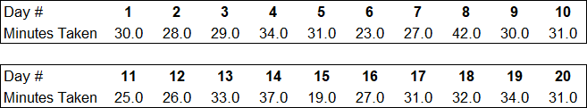 Source: Upstox
The first step is to calculate the average or the mean of the data. You had previously estimated that it took around 30 minutes each day. The way to calculate the average is to add all the observations together and then divide by the number of observations. The formula below shows this as we add all of the travel times together in the numerator. In the denominator, we have the number of observations or in this case, 20 days.
Illustration 2
 Source: Upstox
The mean travel time is, in fact, exactly 30 minutes. The next step is to determine what is known as the ‘standard deviation’ or the average distance from the mean. In the chart below, we plot all of our travel observations. The y-axis on the chart is the number of minutes taken to get to the office.
In the animation, we highlight the mean value of 30 minutes; this line cuts through the approximate centre of the scattered data points. For each one of these data points, we want to calculate the difference between the observation and the mean. For example, if the observation is 34, then the difference for this data point is +4 since the mean is 30. The animation below shows a few examples of calculating the difference between an observation of travel time and the mean of the travel times.
Illustration 3
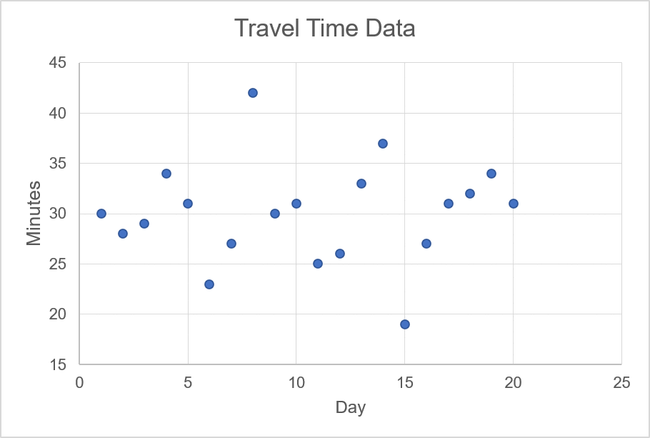 Source: Upstox
Once you calculate the difference between each observation and the mean, you need to then:
- Square the difference of the values.
- Then add those values together.
In the table below, we carry forward the data from Illustration 1 and then perform the difference and squaring calculations.
Illustration 4
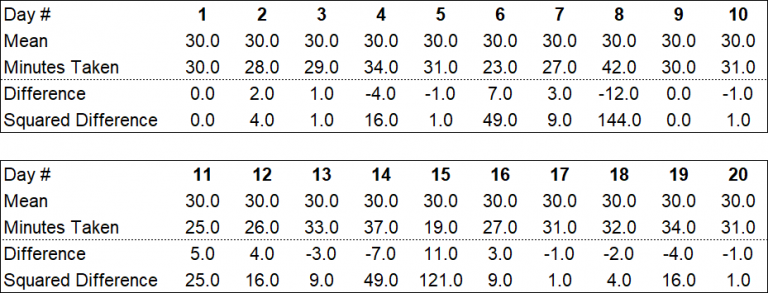 Source: Upstox
If you add all of the values in the ‘squared difference’ rows, you will get 476.0.
The next step is to divide this total by the number of observations minus 1. The number of observations was 20, so we divide 476 by 19, which results in a value of 25.05.
The last step is to take the square root of this number. The square root of 25.05 is 5.005. This is the standard deviation.
Recap: How do you calculate standard deviation?
So, let’s review the steps we used to get to the standard deviation.
- Subtracting the average value from each of the observations.
- Squaring each value (the difference) from step #1.
- Adding up all the values from step #2.
- Subtract 1 from the number of observations.
- Divide the result from step #3 by the result from step #4.
- Calculate the square root of the result from step #5.
So far, we only discussed the manual way to calculate standard deviation (or historical volatility). The good news is that we don’t need to manually calculate the standard deviation as well as the mean – we can use Excel. You simply use the formula ‘=STDEV.S(range of values)’ where the “range of values” are the cells containing the data points you want to analyse. In the illustration below, we use excel to determine the standard deviation instead of manually calculating it.
Illustration 5
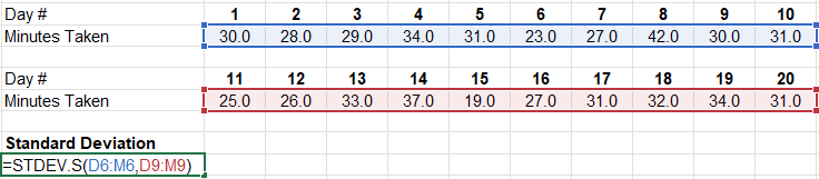 Source: Upstox
While not shown in the illustration, you can also use Excel to calculate the average by using the average or mean. This formula is ‘=AVERAGE(range of values)’.
Key Formula:
- Standard Deviation Excel Formula: = STDEV.S(range of values)Average ##### Excel Formula: =AVERAGE(range of values)
Interpretation of Standard Deviation
So how do you interpret this? In our example, you calculated that the average time to commute to work is 30 minutes. The standard deviation, or the average dispersion from the mean, is 5. We saw commute times that were both above and below the mean so it only makes sense that we can ‘quote’ the standard deviation in relation to the average. If we want to provide a more accurate representation of what our commute time is, we can say that it takes 30 +/- 5 minutes to commute to work.
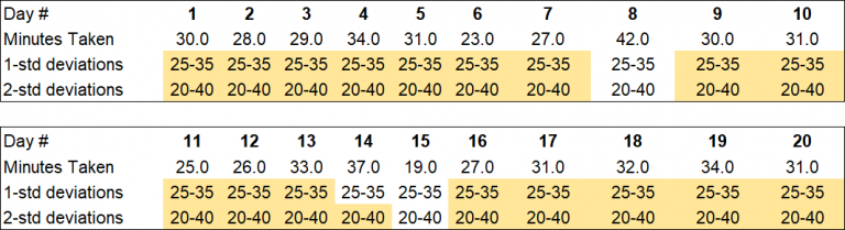
Here, the ‘5’ is one standard deviation from the mean of 30. Two standard deviations from the mean would be ‘10’ in our example. Three standard deviations would be ‘15’ and so forth. Returning to our data table, we’ve added rows that show the ranges of 1- and 2-standard deviations surrounding the mean value of 30. We are highlighting where the ranges of the 1- and 2-standard deviations include the observation.
For example, on day 3, the observation of ‘29’ is found both within the 1-standard deviation range of 25-35 and 2-standard deviation range of 20-40. However, on day 14, the observation is not found in the 1-standard deviation range but is within the 2-standard deviation range. Observations on day 8 and day 15 aren’t found in either the 1- or 2-standard deviation range. As you can see, the 2-standard deviation includes more of the observations than the 1-standard deviation range.
Illustration 6
 Source: Upstox
When you use standard deviation with larger datasets, you can use it to approximate how much of the data will be included within the range. With the markets, there is historical price and return data for securities like stocks, options, and futures. You can use this historical data to calculate average returns as well as the standard deviation of those returns. As we saw in illustration 6, 2-standard deviations will include more of the historical data within it. Specifically:
- 1-standard deviation plus or minus from the mean value will include approximately 68% of observations of the data sample
- 2-standard deviations plus or minus from the mean value will include approximately 95% of observations of the data sample
- 3-standard deviations plus or minus from the mean value will approximately include 99.9% of observations of the data sample
Let’s look at a quick example. Assume you find a stock’s daily returns for the last 5 years. Historically, this stock has returned 0.01% each day with a standard deviation of 1.50%. This means that the stock could likely move +1.51% to -1.49% each day. Of course, past performance isn’t predictive of the future but maybe it is in this case. Therefore, on the majority of days – about 68% of them – the daily return will fall between +1.51% and -1.49%. The other days will see returns that are more variable and will be higher than 1.51% or lower than -1.49%.
This could be used to help a trader or investor understand the risks associated with a potential trade. If you wanted to understand more about the potential daily returns, you could use 2-standard (or 3) deviations. In this example, 2-standard deviations would provide a range of +3.01% to -2.99%. This range covers approximately 95% of historical observations. If history is predictive of the future, then on the vast majority of trading days, the return for this stock will fall within +3.01% and -2.99%.
Again, history is not predictive of the future but historical data can be used as a guardrail to understand potential risks and help in developing your trading plan. When assessing past returns of securities, in particular for options trading, standard deviation is known as ‘historical volatility’ or ‘realised volatility’. We will discuss more about this in the next lesson.
Summary
- The mean is a statistical measure and is the average or expected value of a data set.
- The standard deviation is a statistical measure representing how much the data is dispersed around the mean.
- Standard deviation can be used to help traders assess potential return risks associated with a security.
- 1-standard deviation around a mean value will include about 68% of observations of a data set.
- 2-standard deviations around a mean value will include about 95% of observations of a data set.
- 3-standard deviations around a mean value will include about 99.9% of observations of a data set.
Is this chapter helpful?
- Home/
- Introduction to Standard Deviation